Earthquake Size
Earthquake Magnitude The magnitude is the most often cited measure of an earthquake's size, but it is not the only measure, and in fact, there are different types of earthquake magnitude. Early estimates of earthquake size were based on non-instrumental measures of the earthquakes effects. For example, we could use values such as the number of fatalities or injuries, the maximum value of shaking intensity, or the area of intense shaking. The problem with these measures is that they don't correlate well. The damage and devastation produced by an earthquake will depend on its location, depth, proximity to populated regions, as well as its "true" size. Even for earthquakes close enough to population centers values such as maximum intensity and the area experiencing a particular level of shaking did not correlate well.
With the invention and deployment of seismometers it became possible to accurately locate earthquakes and measure the ground motion produced by seismic waves.
 |
| The development and deployment of seismometers lead to many changes in earthquake studies, magnitude was the first quantitative measure of earthquake size based on seismograms. The maximum or "peak" ground motion is defined as the largest absolute value of ground motion recorded on a seismogram. In the example above the surface wave has the largest deflection, so it determines the peak amplitude. |
Richter's Magnitude Scale
In 1931 a Japanese seismologist named Kiyoo Wadati constructed a chart of maximum ground motion versus distance for a number of earthquakes and noted that the plots for different earthquakes formed parallel, curved lines (the larger earthquakes produced larger amplitudes). The fact that earthquakes of different size generated curves that were roughly parallel suggested that a single number could quantify the relative size of different earthquakes.In 1935 Charles Richter constructed a similar diagram of peak ground motion versus distance and used it to create the first earthquake magnitude scale (a logarithmic relationship between earthquake size and observed peak ground motion). He based his scale on an analogy with the stellar brightness scale commonly used in astronomy which is also similar to the pH scale used to measure acidity (pH is a logarithmic measure of the Hydrogen ion concentration in a solution).
 |
| Sample of the data used by Richter to construct the magnitude scale for southern California. The symbols represent observed peak ground motions for earthquakes recorded during January of 1932 (different symbols represent different earthquakes). The dashed lines represent the reference curve for the decrease in peak-motion amplitude with increasing distance from the earthquake. A magnitude 3.0 earthquake is defined as the size event that generates a maximum ground motion of 1 millimeter (mm) at 100 km distance. |
 |
| Example seismogram recorded on a Wood-Anderson short period seismogram. The top waveform shows the broad-band displacement, the lower trace shows the corresponding ground motion that would register on a Wood-Anderson seismograph. |
Thus originally, Richter's scale was specifically designed for application in southern California. Richter's method became widely used because it was simple, required only the location of the earthquake (to get the distance) and a quick measure of the peak ground motion, was more reliable than older measures such as intensity. It became widely used, well established, and forms the basis for many of the measures that we continue to use today. Generally the magnitude is computed from seismographs from as many seismic recording stations as are available and the average value is used as our estimate of an earthquake's size.
We call the Richter's original magnitude scale ML (for "local magnitude"), but the press usually reports all magnitudes as Richter magnitudes.
Teleseismic Magnitude Scales
To study earthquakes outside southern California, Richter extended the concepts of his local magnitude scale for global application. In the 1930's through the 1950's together with Beno Gutenberg, Richter constructed magnitude scales to compare the size of earthquakes outside of California. Ideally they wanted a magnitude scale that gave the same value if the earthquake is recorded locally or from a great distance. That way you could compare the seismicity of earthquakes in different parts of Earth. But the extension of methods to estimate the local magnitude is complicated because the type of wave generating the largest vibrations and the period of the largest vibrations recorded at different distances from an earthquake varies. Near the earthquake the largest wave is a short-period S-wave, at greater distances longer-period surface waves become dominant.To exploit the best recorded signal (the largest) magnitude scales were developed for "teleseismic" (distant) observations using P waves or Rayleigh waves. Eventually the teleseismic P-wave scale became known as "body-wave magnitude" and the Rayleigh wave based measure came to be called "surface-wave magnitude". The surface-wave magnitude is usually measured from 20s period Rayleigh waves, which are very well transmitted along Earth's surface and thus usually well observed.
 |
| Gutenberg and Richter developed two magnitudes for application to distant earthquakes: mb is measured using the first five seconds of a teleseismic (distant) P-wave and Ms is derived from the maximum amplitude Rayleigh wave. |
Problems with Magnitude Scales
There are several problems associated with using magnitude to quantify earthquakes, and all are a direct consequence of trying to summarize a process as complex as an earthquake in a single number. First, since the distance corrections depend on geology each region must have a slightly different definition of local magnitude. Also, since at different distances we rely on different waves to measure the magnitude, the estimates of earthquake size don't always precisely agree. Also, deep earthquakes do not generate surface waves as well as shallow earthquakes and magnitude estimates based on surface waves are biased low for deep earthquakes.Also, measures of earthquake size based on the maximum ground shaking do not account for another important characteristic of large earthquakes - they shake the ground longer. Consider the example shown in the diagram below. The two seismograms are the P-waves generated by magnitude 6.1 and 7.7 earthquakes from Kamchatka. The body-wave magnitude for these two earthquakes is much closer because the rule for estimating body-wave magnitude is to use the maximum amplitude in the first five seconds of shaking. As you can see, the difference in early shaking between the two earthquakes is much less than the shaking a little bit later which indicates the larger difference in size.
 |
| Teleseismic (distant) P-waves generated by two earthquakes in Kamchatka and recorded at station CCM, Cathedral Caves, MO, US. The signals that would be recorded on a on a short-period seismometer are shown using the same scale. The time is referenced to the onset of rupture for each earthquake. |
Earthquake Dimensions - Rupture Size and Offset
Another measure of earthquake size is the area of the fault that slipped during the earthquake. During large earthquakes the part of the fault that ruptures may be hundreds of kilometers long and 10s of kilometers deep. Smaller earthquake rupture smaller portions of the fault. Thus the area of the rupture is an indicator of the earthquake size. |
| The size of the area that slips during an earthquake is increases with earthquake size. The shaded regions on the fault surface are the areas that rupture during different size events. The largest earthquakes generally rupture the entire depth of the fault, which is controlled by temperature. The temperature increases with depth to a point where the rocks become plastic and no longer store the elastic strain energy necessary to fail suddenly. |
Another measure of an earthquake size is the dimension of the offset produced during an earthquake - that is, how far did the two sides move? Small earthquakes have slips that are less than a centimeter, large earthquakes move the rocks about 10-20 meters.
Seismic Moment and Moment Magnitude
Seismic moment is a quantity that combines the area of the rupture and the amount of fault offset with a measure of the strength of the rocks - the shear modulus m.For scientific studies, the moment is the measure we use since it has fewer limitations than the magnitudes, which often reach a maximum value (we call that magnitude saturation).
To compare seismic moment with magnitude, Mw , we use a formula constructed by Hiroo Kanamori of the California Institute of Seismology:
Magntiude Summary
The symbols used to represent the different magnitudes areGiant Earthquakes
The seismic moment and moment magnitude give us the tool we need to compare the size of the largest quakes. We find that the "moment release" in shallow earthquakes throughout the entire century is dominated by several large subduction zone earthquake sequences. First, let's compare the amount of energy released in the different plate settings:
or we can just compare the largest four earthquakes (those with magnitudes greater than 9) with all the other shallow earthquakes.

Back to EAS 193 Home | Ammon's Home | Department of Geosciences
Prepared by: Charles J. Ammon
How earthquake magnitude scales work
February 16, 2012
by Paul Bodin
We're generally aware that we can barely feel an M3 earthquake, an M6 event can cause some damage, and an M9 can wreak havoc on an entire coast. But what do those numbers mean, and why do seismologists talk about several different magnitude scales?
Here's a dirty little secret: most seismologists hate to talk about magnitude scales with non-seismologists, for several good and related reasons. First, the whole concept of magnitude reduces a complex and variable process--slip on fault patches with differing strength and frictional properties driven by non-uniformly stressed rocks--to a single number. Second, magnitudes are interpretations derived from quantitative measurements (of ground motion recorded on seismographs), not actual measurements themselves. And third, non-seismologists frequently are impatient with the uncertainties arising from the two reasons just stated. Often folks focus on differences between magnitude estimates for the same earthquake reported by different methods and/or organizations, or magnitude estimates that change in time, as being evidence of some vast conspiracy of government scientists to hide evidence of either ineptitude or deceit (so we seismologists are often a bit defensive).
Chuck Ammon at Penn State provides a good basic overview of how earthquake magnitudes are determined.
Here we just want to point out a few basic ideas that will help non-seismologists understand some of the technical issues the next time a journalist is making a big deal about, say, an earthquake that PNSN reports as an M3.2 and the NEIC (National Earthquake Information Center in Golden, CO) reports as an M3.5 (or whatever). First of all, of course, we're right! Well, so may be the NEIC. As right as anyone can be, at any rate, and here's why. Oh...and I'm only going to talk about what is called Local Magnitude, a measure based on the largest signal (peak amplitude) measured on seismographs. Other magnitude scales are based on the duration of shaking or matching the seismic waveform wiggle-for-wiggle to a model. Those are for a different blog (and our soon-to-be-published "Discovery & Outreach" wepages) and they are all, ultimately tied to the Local Magnitude, (or ML).
Back in the day (1930s), magnitudes started as simply the logarithm of the amplitude of the largest oscillations written on a specific seismograph at CalTech (a Wood-Anderson torsion seismograph measuring horizontal motion, if you must know!). The instrument Charles Richter used was the standard. Really for no other reason than that he had it and so he used it. He used the logarithm of the amplitude because there was such a large range of amplitudes that the compression of scale you get from taking logs made things easier to plot. Some darned earthquake that was 100 km away, made a trace with a peak displacement of 1 mm on his seismograph and he called that the standard earthquake--magnitude 1. An earthquake at the same distance that made a displacement of 10 mm was a magnitude 2, 100 mm was magnitude 3, and so on. "Smaller" earthquakes closer to the lab or "larger" earthquakes more distant might produce the same peak amplitude, so the formula includes a distance correction for earthquakes not at the standard distance. This explains an enduring mystery to many folks--negative magnitudes. An earthquake that wrote a record with a peak displacement of 0.1 mm would be a magnitude 0, right? And if that earthquake were closer than 100 km, well ... it would have a negative magnitude. Remember: Magnitudes are a relative size estimate. Nothing absolute about them (but, perhaps, Charlie Richter's arbitrary "standard" earthquake and seismograph); no physical units ascribed to them.
But why do I feel compelled to encase the terms "smaller" and "larger" in quotes so much? Well, because earthquakes, like elephants or people, get bigger in different ways. Both a basketball player and a sumo wrestler are clearly "bigger" than a child or a short lightweight person, but that doesn't make them equally big or similar in appearance. Bigness, it turns out, may be in the eye of the beholder. When physical scientists wander into pickles like this they usually turn to the concept of energy to compare things. And so, too, with earthquakes.

An earthquake is slippage of one side of a fault against the other side of a fault. It turns out that a more robust measurement of the energy it releases is the distance it slips times the area that did the slipping. An M6 earthquake, for example, might involve a meter of slip on a fault plane 10 km by 10 km. The simplest measure of the size (as energy) of the resulting earthquake, called the moment, is proportional to the area (length times width) of the fault, times the average amount of slip. And since fault ruptures range from cms to hundreds of km in dimension (and slip from millimeters to meters), the difference in moment between the smallest and largest earthquakes varies by many, many orders of magnitude (getting the idea how the name "magnitude" for earthquake size originated?), and those non-logarithmic numbers are inappropriate to give to the public, most of whom (like me) are buffaloed by balancing a nice linear checking account balance. (Imagine: Nicely coiffed news reporter asks "Dr. Bodin, how big was the earthquake?", frowzy grumpy seismologist answers: "Oh it was approximately 54,000,000,000,000,000 newton-meters, give or take a few million, Bob". You see the problem....)
There are invariably devils amongst the details. It turns out that earthquakes radiate different amounts of energy as seismic waves in different directions, for example. (One way we tell the orientation of the fault that broke). And even the direction a rupture propagates can lead to different amplitudes in different directions (called "rupture directivity"). For this reason the number and geometry of stations around an earthquake, and how you average them (remember---magnitude is ONE number!) is important in coming out with that one number everyone craves. Also, the soil or rock that a seismometer is placed on can de-amplify seismic motions, or even amplify them, so each site should have a "site correction" in addition. Also, the background noise at the time of the earthquake signal's passing can add to, or subtract from, the peak amplitude measured. Another reason to average in as many station estimates as you can. You get the idea.
So it's really quite easy to see how early on, we compute an automatic ML without looking at the traces, but then upon review decide that we should throw out channels that are really too noisy, or that may have been really broken at the time. And that changes the magnitude estimate to one we're more sure of. And how NEIC and/or PGC in Canada, and/or CISN in California look at the THEIR stations and compute a different magntitude value. As a rule of thumb, though, I'd say most seismologists aren't at all surprised by differences of up to .5 magnitude units in early estimates. However, when different organizations report the same magnitude type that vary by more than that after about 1/2 an hour from an earthquake, there was probably a more significant error involved.
https://pnsn.org/blog/2012/02/16/how-earthquake-magnitude-scales-work
Here's a dirty little secret: most seismologists hate to talk about magnitude scales with non-seismologists, for several good and related reasons. First, the whole concept of magnitude reduces a complex and variable process--slip on fault patches with differing strength and frictional properties driven by non-uniformly stressed rocks--to a single number. Second, magnitudes are interpretations derived from quantitative measurements (of ground motion recorded on seismographs), not actual measurements themselves. And third, non-seismologists frequently are impatient with the uncertainties arising from the two reasons just stated. Often folks focus on differences between magnitude estimates for the same earthquake reported by different methods and/or organizations, or magnitude estimates that change in time, as being evidence of some vast conspiracy of government scientists to hide evidence of either ineptitude or deceit (so we seismologists are often a bit defensive).
Chuck Ammon at Penn State provides a good basic overview of how earthquake magnitudes are determined.
Here we just want to point out a few basic ideas that will help non-seismologists understand some of the technical issues the next time a journalist is making a big deal about, say, an earthquake that PNSN reports as an M3.2 and the NEIC (National Earthquake Information Center in Golden, CO) reports as an M3.5 (or whatever). First of all, of course, we're right! Well, so may be the NEIC. As right as anyone can be, at any rate, and here's why. Oh...and I'm only going to talk about what is called Local Magnitude, a measure based on the largest signal (peak amplitude) measured on seismographs. Other magnitude scales are based on the duration of shaking or matching the seismic waveform wiggle-for-wiggle to a model. Those are for a different blog (and our soon-to-be-published "Discovery & Outreach" wepages) and they are all, ultimately tied to the Local Magnitude, (or ML).
It's Beno Guttenberg and Charlie Richter's fault...
Back in the day (1930s), magnitudes started as simply the logarithm of the amplitude of the largest oscillations written on a specific seismograph at CalTech (a Wood-Anderson torsion seismograph measuring horizontal motion, if you must know!). The instrument Charles Richter used was the standard. Really for no other reason than that he had it and so he used it. He used the logarithm of the amplitude because there was such a large range of amplitudes that the compression of scale you get from taking logs made things easier to plot. Some darned earthquake that was 100 km away, made a trace with a peak displacement of 1 mm on his seismograph and he called that the standard earthquake--magnitude 1. An earthquake at the same distance that made a displacement of 10 mm was a magnitude 2, 100 mm was magnitude 3, and so on. "Smaller" earthquakes closer to the lab or "larger" earthquakes more distant might produce the same peak amplitude, so the formula includes a distance correction for earthquakes not at the standard distance. This explains an enduring mystery to many folks--negative magnitudes. An earthquake that wrote a record with a peak displacement of 0.1 mm would be a magnitude 0, right? And if that earthquake were closer than 100 km, well ... it would have a negative magnitude. Remember: Magnitudes are a relative size estimate. Nothing absolute about them (but, perhaps, Charlie Richter's arbitrary "standard" earthquake and seismograph); no physical units ascribed to them.

What do you mean by "bigger"?
But why do I feel compelled to encase the terms "smaller" and "larger" in quotes so much? Well, because earthquakes, like elephants or people, get bigger in different ways. Both a basketball player and a sumo wrestler are clearly "bigger" than a child or a short lightweight person, but that doesn't make them equally big or similar in appearance. Bigness, it turns out, may be in the eye of the beholder. When physical scientists wander into pickles like this they usually turn to the concept of energy to compare things. And so, too, with earthquakes.
An earthquake is slippage of one side of a fault against the other side of a fault. It turns out that a more robust measurement of the energy it releases is the distance it slips times the area that did the slipping. An M6 earthquake, for example, might involve a meter of slip on a fault plane 10 km by 10 km. The simplest measure of the size (as energy) of the resulting earthquake, called the moment, is proportional to the area (length times width) of the fault, times the average amount of slip. And since fault ruptures range from cms to hundreds of km in dimension (and slip from millimeters to meters), the difference in moment between the smallest and largest earthquakes varies by many, many orders of magnitude (getting the idea how the name "magnitude" for earthquake size originated?), and those non-logarithmic numbers are inappropriate to give to the public, most of whom (like me) are buffaloed by balancing a nice linear checking account balance. (Imagine: Nicely coiffed news reporter asks "Dr. Bodin, how big was the earthquake?", frowzy grumpy seismologist answers: "Oh it was approximately 54,000,000,000,000,000 newton-meters, give or take a few million, Bob". You see the problem....)
Devlish details...
There are invariably devils amongst the details. It turns out that earthquakes radiate different amounts of energy as seismic waves in different directions, for example. (One way we tell the orientation of the fault that broke). And even the direction a rupture propagates can lead to different amplitudes in different directions (called "rupture directivity"). For this reason the number and geometry of stations around an earthquake, and how you average them (remember---magnitude is ONE number!) is important in coming out with that one number everyone craves. Also, the soil or rock that a seismometer is placed on can de-amplify seismic motions, or even amplify them, so each site should have a "site correction" in addition. Also, the background noise at the time of the earthquake signal's passing can add to, or subtract from, the peak amplitude measured. Another reason to average in as many station estimates as you can. You get the idea.
So it's really quite easy to see how early on, we compute an automatic ML without looking at the traces, but then upon review decide that we should throw out channels that are really too noisy, or that may have been really broken at the time. And that changes the magnitude estimate to one we're more sure of. And how NEIC and/or PGC in Canada, and/or CISN in California look at the THEIR stations and compute a different magntitude value. As a rule of thumb, though, I'd say most seismologists aren't at all surprised by differences of up to .5 magnitude units in early estimates. However, when different organizations report the same magnitude type that vary by more than that after about 1/2 an hour from an earthquake, there was probably a more significant error involved.
https://pnsn.org/blog/2012/02/16/how-earthquake-magnitude-scales-work